Does a Rising Tide Really Lift All Boats?

Python

Hypothesis Testing

Peer Analysis

Equity Research

Statistics

Confidence Intervals

Using hypothesis testing and peer analysis to ascertain the fair value of public companies

Published

December 24, 2023

Problem with Ratio & Comparison Analysis

You might have encountered the expression “a rising tide lifts all boats,” often attributed to ‘friendly’ politicians or laissez-faire economists. This phrase hints at the idea that overall growth or prosperity benefits everyone, irrespective of individual circumstances. I aim to examine whether this concept holds true in the context of stocks…well kind of. That question and idea has some what morphed into me answering a much different question.

As a financial analyst, various methods are employed to assess the value of equity investments. In this discussion, I’d like to focus on ratio analysis, particularly the comparison of valuation ratios among companies.

The significance of ratio analysis becomes evident when considering the comparative aspect. A ratio, at its core, represents the division of two numbers. The premise is that companies with similar traits (business models, profitability, debt, etc.) should carry similar valuations. For instance, comparing Apple, a mature tech company with a P/E ratio of 24.5, to Microsoft with a P/E ratio of 37.2, or assessing JPM’s P/B ratio of 1.69 against Bank of America’s 1.03, highlights the diverse interpretations drawn by analysts. One might view Apple as undervalued and choose to invest, while another might see it as fairly priced and consider shorting Microsoft. Detailed financial analysis is imperative in reaching such conclusions.

In this simplified illustration, ratio analysis involves evaluating multiple comparable companies to identify potential value in stocks. However, a fundamental challenge arises: is Company A undervalued, or is its peer overvalued? The solution often involves comparing with multiple peers. For instance, even after analyzing five similar banks, an analyst might still perceive JP Morgan and Microsoft as overvalued and opt to short the stocks. But historical data might reveal that these companies consistently maintain higher earnings and valuation multiples compared to their peers.

So, what’s the dilemma for the analyst? How can we value a company based on its peers when those peers possess similar yet differing valuations? This is precisely what we will delve into in this discussion.

Methodology & Overview

The typical advice for valuing a company based on a ratio involves “comparing it to its peers.” However, companies are inherently different, leading to varying valuation ratios due to factors like profitability, growth, business model, and debt. This raises the fundamental question: How can we use ratio analysis to value similar companies when their valuations will inevitably differ?

The solution lies in not directly comparing the ratios themselves, but rather in assessing the differences in ratios between companies over time. This approach helps determine whether the current valuation is statistically higher or lower than expected.

Our approach involves stating null and alternative hypotheses, followed by calculating the differences in valuation ratios between a target company and its peer group over a period. Subsequently, constructing a confidence interval will establish a fair value range, enabling us to ascertain if the target company is overvalued or undervalued compared to its peers.

Assumptions

That the current peer group selected is priced at fair value (not under or over valued). This assumption becomes easier to make the larger the sample becomes. (subjective to the analyst)
There is no non-systematic public material information (good or bad) that would reasonably cause a deviation to exist or persist in the valuation of the target or peer group. (subjective to the analyst)

This is my first attempt at this method to to value equities so future updates will hopefully refine the process & correct any errors but, for now the journey of discovery is exciting no matter the outcome.

Hypothesis

Null Hypothesis (H0): The Target company’s current valuation ratio difference from its peers’ valuation ratio is equal to the historical average difference. H0: μ_difference = 2.128

Alternative Hypothesis (H1): The Target company’s current difference from its peers’ valuation is NOT equal to the historical average difference. H1: μ_difference ≠ 2.128

Lets Get Some Data!

Packages Used

import plotly.express as px
import plotly.graph_objects as go

import requests
import pandas as pd
import numpy as np
import scipy.stats as stats
from scipy.stats import ttest_1samp

from datetime import datetime
from datetime import timedelta
import warnings

#only for demo purposes.
from rich import print

#key = "apikey"

I love functions so lets make some to get some data from the FMP API (Financial Modeling Prep).

#Gets the current P/B figure for a stock
def get_current_ratio(stock_symbols, key=key):
    ratio = {}

    for symbol in stock_symbols:
        request = f'https://financialmodelingprep.com/api/v3/key-metrics-ttm/{symbol}?apikey={key}'
        data = requests.get(request).json()
        data = pd.DataFrame(data)
        pe = data.ptbRatioTTM.astype(float)
        ratio[symbol] = pe

    return ratio


#Gets 20 quarters of P/B figures for a list of stocks
def get_historical_ratio(stock_symbols, key=key):
    ratio = {}

    for symbol in stock_symbols:
        request = f'https://financialmodelingprep.com/api/v3/ratios/{symbol}?period=quarterly&limit=20&apikey={key}'
        data = requests.get(request).json()
        data = pd.DataFrame(data)
        pe = data.priceToBookRatio.astype(float)
        ratio[symbol] = pe

    return ratio

We will be retrieving 20 quarters of data for 6 peer companies (PSX, MPC, VLO, DINO, PBF, PARR) and 1 target company (SUN)

#Set the peer group and target company
peer_symbols = ["PSX","MPC","VLO","DINO","PBF","PARR"]
target_symbol = ["SUN"]

Now Lets call our functions and get the data. We will be retrieving current and historical for both the target and peer group so be careful not to get the two confused. For this project I labeled historical “_hist” and the current data as “_curr”

Current P/B Data

#Current data or today's P/B ratio's
peer_curr = get_current_ratio(peer_symbols)
target_curr = get_current_ratio(target_symbol)

peer_curr = pd.DataFrame(peer_curr)
target_curr = pd.DataFrame(target_curr)

Output

index	SUN
0	4.4141

index	PSX	MPC	VLO	DINO	PBF	PARR
0	1.9417	2.2834	1.7711	0.9867	0.8173	2.0739

Historical P/B Data

peer_hist = get_historical_ratio(peer_symbols)
target_hist = get_historical_ratio(target_symbol)

peer_hist = pd.DataFrame(peer_hist)
target_hist = pd.DataFrame(target_hist)

.head() Output

index	PSX	MPC	VLO	DINO	PBF	PARR
2023-09-30	1.7319	2.3056	1.9040	0.9946	0.9657	2.0204
2023-06-30	1.4498	1.8965	1.6244	0.8838	0.8485	1.7483
2023-03-31	1.5578	2.2397	2.0624	1.0200	1.0600	1.9766
2022-12-31	1.6651	1.9660	2.0460	1.0332	1.0199	2.1543
2022-09-30	1.3763	1.8652	1.7572	1.1694	1.0179	1.7864

index	SUN
2023-09-30	3.4872
2023-06-30	3.6654
2023-03-31	3.6893
2022-12-31	3.8358
2022-09-30	3.3377

Visualize The Data

Let’s visually represent the data to assess whether it is worth continuing with the current selection and see what type of data cleaning will be necessary. However, before proceeding, it’s essential to incorporate a date range and merge our target and peer historical data into a single dataframe for easier visualization on the plotly graph.

#generate the dates, using start, periods and frequency
rng = pd.date_range(start='12/31/2018', periods = 20, freq="Q").sort_values(ascending=False)

#add date as index to historical data
peer_hist.index = rng
target_hist.index = rng

#For current Data add today's date
peer_curr.index = [datetime.today().date()] * len(peer_curr)
target_curr.index = [datetime.today().date()] * len(target_curr)

#create a data set with target and peers historical data
all_hist = pd.concat([peer_hist, target_hist], axis=1)

.head() Output

index	PSX	MPC	VLO	DINO	PBF	PARR	SUN
2023-09-30	1.7320	2.3056	1.9040	0.9946	0.9657	2.0204	3.4872
2023-06-30	1.4498	1.8965	1.6244	0.8838	0.8485	1.7483	3.6654
2023-03-31	1.5578	2.2397	2.0624	1.0200	1.0600	1.9766	3.6893
2022-12-31	1.6651	1.9660	2.0460	1.0332	1.0199	2.1543	3.8358
2022-09-30	1.3763	1.8652	1.7572	1.1694	1.0179	1.7864	3.3377

Clean The Data

Excellent, our data doesn’t contain any zero values to eliminate or NaNs. This is precisely why I opted for P/B, given its reduced susceptibility to being zero. However, if it does reach that point, it’s a strong indicator that the stock might not warrant serious consideration. That said, delving into this aspect warrants a separate discussion.

Yet, there’s a challenge with the data: PARR’s P/B value surged during the pandemic while the others remained relatively stable. This discrepancy might skew our results, so lets drop PARR from the dataset.

Moving forward, future attempts will involve a more refined peer selection process. This process will involve determining the stocks that exhibit the closest movement with the target firm, employing methods such as betas or correlations.

peer_hist.drop('PARR', axis=1, inplace=True)
peer_curr.drop('PARR', axis=1, inplace=True)

#1) if using ratios with negative values replace negatives with 0 or remove from dataset.
peer_hist = peer_hist.clip(lower=0)

Dataset without PARR

Calculate Statistics

Now lets get some general statistics about the data

Calculate Averages

#Calculate the mean average of the current data
peer_avg_curr = peer_curr.mean(axis='columns')
peer_avg_curr = pd.DataFrame(peer_avg_curr, columns=['Peer Avg'])

index	Peer Avg
2023-12-27	1.6461

peer_avg_hist = peer_hist.mean(axis='columns')
peer_avg_hist = pd.DataFrame(peer_avg_hist, columns=['Peer Avg'])

.head() Output

index	Peer Avg
2023-09-30	1.6537
2023-06-30	1.4085
2023-03-31	1.6527
2022-12-31	1.6474
2022-09-30	1.4954

Current & Historical P/B of SUN and Peer Group Average

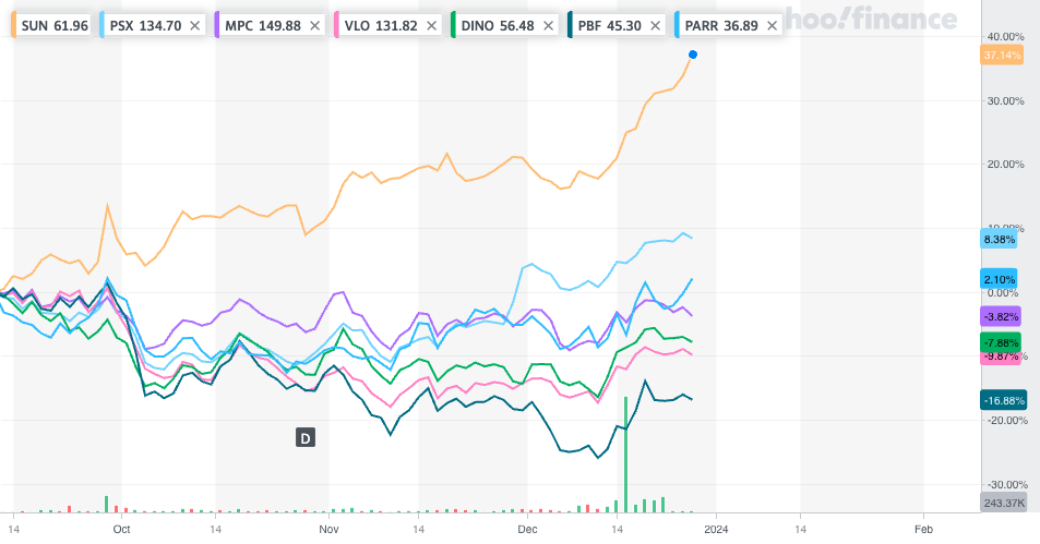
As observed, they don’t exhibit perfect alignment, yet there’s a noticeable trend of moving in generally the same directions concurrently and with comparable magnitudes through most of the historical data. However, after the 19th observation (9-30-23), the target firm SUN’s P/B ratio shows a notable surge while its peers have maintained a more stable trajectory. It’s worth exploring whether there have been any alterations in SUN’s business that could justify this deviation or rise. If no significant changes are found, this anomaly might signify an unwarranted surge in the stock price or a decrease in the book value without a corresponding decline in the stock price. The chart below shows that SUN’s price has moved up 37% while its peers have risen at a more moderate level and many have even declined.

Calculate the Differences

The next step involves computing the variance between the target and the peer average for each observation. This calculation will serve as the foundation for determining whether the target firm (SUN) is either overvalued or undervalued in comparison to its peers.

#Current difference
diff_curr = pd.DataFrame(abs(target_curr['SUN'] - peer_avg_curr['Peer Avg']), columns=['Difference'])

print(diff_curr)

#Historical difference
diff_hist = pd.DataFrame(abs(target_hist['SUN'] - peer_avg_hist['Peer Avg']), columns=['Difference'])

print(diff_hist)

            Difference
2023-12-28      2.9149

            Difference
2023-09-30      1.9069
2023-06-30      2.3248
...                ...
2019-03-31      1.7999
2018-12-31      1.4999

[20 rows x 1 columns]

Calculate Mean Historical Differences

Now find the mean difference in the data before 9/30/2023

#Mean difference
mean_diff_hist = diff_hist.mean()
print(mean_diff_hist)

#Standard deviation of differences
std_hist = diff_hist['Difference'].std()
print("std:", std_hist)

Difference    2.128
dtype: float64

std: 0.3906206520896308

At this stage, a one-sample t-test would typically be conducted on the data. However, for brevity and because the insight of a t-test isn’t as applicable in this scenario where the objective is to determine the fair value, we’ll opt for using a confidence interval instead.

Build Confidence Interval

With all the data now calculated, it’s time to construct a confidence interval and assess whether the current value of our target company exceeds its normal range relative to its peers.

Scipy stats makes this a one line operation :)

stats.t.interval(confidence=0.999, df=len(diff_hist) - 1, loc=mean_diff_hist, scale=stats.sem(diff_hist))

(array([1.78879906]), array([2.46719459]))

Alternatively, breaking it down gives us the same results

mean_diff_hist = diff_hist.mean()
std_err = stats.sem(diff_hist)

# Calculate confidence interval
confidence_level = 0.999
n = len(diff_hist)
t_value = stats.t.ppf((1 + confidence_level) / 2, n - 1)
margin_of_error = t_value * std_err
confidence_interval = pd.DataFrame([mean_diff_hist - margin_of_error, mean_diff_hist + margin_of_error])
print(confidence_interval)

   Difference
0      1.7888
1      2.4672

Visualize the Confidence Interval

Combine historical differences with current difference.

diff_all = pd.concat([diff_curr, diff_hist], axis=0)

index	Difference
2023-12-27	2.7181
2023-09-30	1.8335
2023-06-30	2.2568
…	…
2019-09-30	1.9139
2019-06-30	1.9175
2019-03-31	1.7938

As we can see the current difference between SUN and the Peer Group average P/B value extends beyond 2.8 which greatly exceeds the confidence interval upper bound of 2.4676.

Estimating Fair Value

Applying the confidence interval to the valuation ratio involves a straightforward process. Given that the CI represents the disparity between the ‘peer group average’ and the ‘target company,’ we add both the upper and lower bounds of the CI to the current peer valuation ratio (p/e, p/b, p/s). While this might initially seem counterintuitive—usually, subtraction is employed to determine the lower bound—recall that we’ve already conducted the subtraction to ascertain the “lower bound difference.” Thus, the addition of both bounds helps establish the range within which the valuation ratio (p/e, p/b, p/s) of the target company is statistically likely to fall. Consequently, this results in defining both a high valuation ratio and a low valuation ratio. At a 99% confidence level, our prediction indicates that the fair value is expected to lie somewhere between these two extremes.

#establishing the upper and lower bounds for the P/B ratio
upper_ratio = peer_avg_curr.iloc[0,0] + confidence_interval.iloc[1,0]
lower_ratio = peer_avg_curr.iloc[0,0] + confidence_interval.iloc[0,0]
print("The current fair value of the target company lies between a P/B value of: ", upper_ratio, " to ",lower_ratio)

The current fair value of the target company lies between a P/B value of:  4.001255588456896  to  
3.3228600564256956

By determining the statistically derived fair P/B range, investors now have a guideline to consider when assessing the valuation of the target company. But lets keep going and calculate the fair value price.

#First get the current price of the target
def get_price(symbol, key=key):

  request = f'https://financialmodelingprep.com/api/v3/quote/{symbol}?apikey={key}'
  data = requests.get(request).json()
  data = pd.DataFrame(data)
  price = data.price.astype(float)

  return price

#Get current price of Target
price_of_target = get_price('SUN')
print(price_of_target)


#Use Algebra to solve for the book value per share
bvps = price_of_target / target_curr.iloc[0,0]
print(bvps)

0    62.45
Name: price, dtype: float64

0    14.0368
Name: price, dtype: float64

The last step involves computing the fair value range by multiplying the previously calculated book value with the upper and lower fair value ratios.

price_low = bvps[0] * lower_ratio
price_high = bvps[0] * upper_ratio
print("The fair value of the target company lies between", round(price_low, 2), "and", round(price_high,2), "dollars per share.", "The target company is currently trading at a P/B of:", price_of_target[0])

The fair value of the target company lies between 46.64 and 56.17 dollars per share. The target company is 
currently trading at a P/B of: 62.45

#Fair value of Target
fair_value_mean = (price_high + price_low) / 2
print("At a fair value of:", round(fair_value_mean, 2) , "the target company is overvalued by:", round(price_of_target[0] - fair_value_mean, 2))

At a fair value of: 51.4 the target company is overvalued by: 11.05

Conclusion

Nice!!! A ton of work but we did it, we now have a fair value rang for SUN based on it’s peers. Remeber there are two main assumptions that go into this model.

That the current peer group selected is priced at fair value (not under or over valued). This assumption becomes easier to make the larger the sample becomes. (subjective to the analyst)
There is no non-systematic public material information (good or bad) that would reasonably cause a deviation to exist or persist in the valuation of the target or peer group. (subjective to the analyst)

Holding these true it safe to assume that SUN is overvalued based on the current model.

Future Updates

I will definitely be coming back to this topic soon after I do some more reading and think on how to refine and perfect the model. Here are just some of the things I am looking to improve upon or add.

t-test using critical value and p-values for significance.
Developing a system to pick peer group based on beta or correlations
MORE DATA!
Using a normal distribution if possible
More data analysis (check for stationary, correlations, trend analysis)
Monte Carlo Simulatio

Problem with Ratio & Comparison Analysis

Methodology & Overview

Hypothesis

Lets Get Some Data!

Current P/B Data

Historical P/B Data

Visualize The Data

Clean The Data

Calculate Statistics

Calculate Averages

Current & Historical P/B of SUN and Peer Group Average

Calculate the Differences

Calculate Mean Historical Differences

Build Confidence Interval

Visualize the Confidence Interval

Estimating Fair Value

Conclusion

Future Updates

Thanks for making it to the end of this very long experiment!